Follow The Bouncing Signal (E)

Signal jamming, noise generation/interference, signal interception, and other malicious RF-related activities have long been part and parcel of the electronic warfare arena. One countermeasure that is widely deployed is frequency hopping spread-spectrum (FHSS) transmission, or rapid and pseudo-random jumps of the carrier frequency in an effort to confound would-be jammers. FHSS transmission poses test and measurement challenges that we'll outline below.

In a scenario in which you're trying to follow a signal as it ducks and weaves from carrier frequency to carrier frequency, your best friend may be your oscilloscope's Trend plotting capabilities (see this earlier post for information on how Trend plots can help with power measurements). Figure 1 shows the fast-Fourier transform (FFT) of a frequency-hopping input signal (F6 in red). Below that is a Trend plot of that FFT's peak frequency as a function of time. A look at the plot tells us that the carrier frequency of our signal peaks, then gradually decreases until it makes an instantaneous step change back to the high frequency. Thus, we gain a history of where the frequency goes on a frequency vs. time axis. Any frequency this signal moves to is recorded in the trend plot, which itself constitutes a waveform on which you can take measurements and perform additional analysis.

Another interesting example of a frequency-hopping signal appears in Figure 2. Again, we can determine the pattern by taking a trend plot of an FFT of the input signal. In this case, the frequency traverses a linear sweep and suddenly breaks into a very different pattern with numerous step changes.

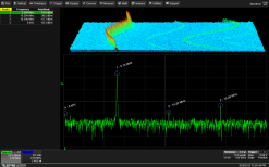
To delve even further into the characteristics of an FHSS signal, we can augment the trend plot with histograms. The histogram can tell us the dwell time of the frequency peak at its various stops. In Figure 3, we can see that it spends a disproportionate amount of time at one frequency. We can determine what percentage of the time it spends at this frequency versus the other values, or we can determine the value for each of the frequencies either as a percentage or a ratio.

For a final example of the breadth of information that can be gleaned from an RF burst, Figure 4 shows a capture of an RF burst (C1 in yellow) with an FFT below it (F6 in red). The parameter x@max, which uses the FFT as its source, shows where the frequency peak is at all times. At bottom left is the plot of pulse amplitude vs. time (F8 in green), while the plot of frequency peak vs. time appears at center right (F7 in blue). At top right is a histogram that gives us the number of occurrences for specific frequencies. The teal trace at lower right simply shows that the oscilloscope is set to trigger on the marker pulse.

Armed with a sufficiently powerful oscilloscope, one can discover many interesting facets of an FHSS signal.

Das ist eine Applikations-Schrift von Teledyne LeCroy.